Recommending blog posts with machine learning

Regular readers of Giant Robots may have noticed that we recently added links to recommended posts at the end of every post on the blog. The intention is to help you find more posts that might be interesting to you. In this blog post I’m going to get a little meta and talk about how we did that.

This blog has been around for more than a decade, and has more than 1,600 posts. That’s a lot of content to curate by hand, so when we wanted to add related posts, we knew we needed an automated solution.

What makes a good related post?

Ideally, the posts we recommend will be on similar topics to the one you just finished reading.

We could consider using tags for this, but that doesn’t give us much to work with. Our average post has 2 or 3 tags, and while there are around 300 tags in total, there are only 47 that we’ve used more than 10 times. If you were looking at a post with a very popular tag—like web, or rails—we’d have a lot of posts with the same tag that we could recommend, but little information to narrow down which of those posts would be a good follow-up to the one you’re reading.

What we need is a more fine-grained approach to identifying the topics covered by each post.

Enter topic modelling

A topic model is a statistical model for discovering topics in a corpus of documents, based on words that commonly appear together. Documents typically cover multiple topics, giving different emphasis to each topic. For example a post that is mostly about Test Driven Development might also touch on some Ruby on Rails concepts in the examples it uses, in which case we’d expect to see lots of words associated with the TDD topic and a scattering of words from the Rails topic.

This can be very useful for finding related posts, because we can search for similarities not just to one topic, but to the whole topic distribution of the post. If you just finished a post that’s mostly TDD with a hint of Rails, we can recommend other posts that focus on TDD and mention Rails.

The gory details

That covers the why and the what, let’s take a look at how.

We opted for a latent Dirichlet allocation (LDA) model, because it’s widely used, implemented by some well-supported libraries, and was something we’d already experimented with for other projects. If you want to understand how the algorithm works, I recommend David Lettier’s Your Easy Guide to Latent Dirichlet Allocation on Medium.

As is often the case with machine learning problems these days, there are great libraries available for the model itself—we used the gensim Python library here—and most of the code we needed to write deals with preparing the data, selecting the right parameters for the model, and using the model’s output.

Preparing the data

As with many natural language processing libraries, gensim expects documents to be represented as a bag of words, which meant there was some pre-processing to do. Each blog post goes through the following stages:

1. We write our posts in Markdown, so each post starts out as a big old Unicode string, something like this:

   '''
   I recently wrote about using [machine learning
   to understand ingredients in recipes][NER]. There's
   no way I could consider every possible format for
   recipe ...
   '''

1. We’re not interested in anything but the raw text, so we can strip out any Markdown formating or HTML tags. In practice, it proved easier to go from Markdown to HTML, and then from HTML to text.

   '''
   I recently wrote about using machine learning
   to understand ingredients in recipes. There's
   no way I could consider every possible format for
   recipe ...
   '''

1. Next we want to split the text into tokens, each of which is an interesting word. Gensim has a simple_preprocess function we used for this. We also used the list of stop words from the Natural Language Toolkit (NLTK) to prevent common words like and, the, but or if from being considered—we don’t want our topics to be confused with irrelevant words that just happen to appear in some posts more often than they appear in others. After this tokenizing step, our example post looks like this:

   ['recently', 'wrote', 'using', 'machine', 'learning',
    'understand', 'ingredients', 'recipes', 'way', 'could',
    'consider', 'every', 'possible', 'format', 'recipe',
    ... ]

1. Some of our tokens are really part of multi-word phrases. In this example, it’s going to be more useful to consider machine learning to be one token instead of an instance of the token machine and a separate instance of the token learning. To account for this we next merge bigrams and trigrams, by using gensim’s phrase model. The result is similar, but some of the tokens have been combined:

   ['recently', 'wrote', 'using', 'machine_learning',
    'understand', 'ingredients', 'recipes', 'way', 'could',
    'consider', 'every', 'possible', 'format', 'recipe',
    ... ]

1. Next up, we want to lemmatize the tokens, so that words with the same root, like recipes and recipe will be treated as the same token. We used spaCy’s lemmatizer. We could have used NLTK here too, but it’s a little more involved than spaCy because NLTK provides various models from different sources, and there’s sometimes manual translation required to go from one to another.

   ['recently', 'write', 'use', 'machine_learn',
    'understand', 'ingredient', 'recipe', 'way', 'could',
    'consider', 'every', 'possible', 'format', 'recipe',
    ... ]

1. In our final filtering step, we use parts of speech tags—also from spaCy—to drop any tokens that aren’t likely to be useful. We’ll keep the nouns, adjectives, verbs, and adverbs, and drop the rest.

   ['recently', 'write', 'use', 'machine_learn',
    'understand', 'ingredient', 'recipe', 'way', 'could',
    'consider', 'possible', 'format', 'recipe',
    ... ]

1. Finally we’re ready to turn this into a bag of words, which is a list of tuples, each containing a word, and the number of times the word occurs in the post.

   [('recently', 1), ('write', 1), ('use', 1), ('machine_learn', 1),
    ('understand', 1), ('ingredient', 1), ('recipe', 2), ('way', 1),
    ('could', 1), ('consider', 1), ('possible', 1), ('format', 1),
    ... ]

In practice gensim uses a Dictionary class, which maps each word to a unique ID. The bag of words representing each post uses the IDs to save storing, passing around, and comparing thousands of bulky Unicode strings.

   # Dictionary.token2id
   {'recently': 0, 'write': 1, 'use': 2, 'machine_learn': 3, ... }

   # Bag of words
   [(0, 1), (1, 1), (2, 1), (3, 1), ... ]

Parameter selection

Once the data was in the right format, we could train the model.

The most important parameter to choose for an LDA topic model is the number of topics. With too few topics, the model won’t really capture the full scope of the blog. With too many topics, the model will learn artificial distinctions that may be present in the words used in the content, but won’t really matter to a reader of the blog. Either way, the recommendations the model makes will suffer.

We took the usual approach: decide on a metric that tells us our model is good, and try various parameter values until we find the one that yields the best result for our chosen metric.

A common metric for topic models is coherence, which is based on the likelihood of the words that make up a topic appearing in the same document. The more likely it is that the topic’s words appear together, the more coherent the topic is.

Conveniently, gensim provides a topic_coherence function that we used to evaluate different models with different numbers of topics.

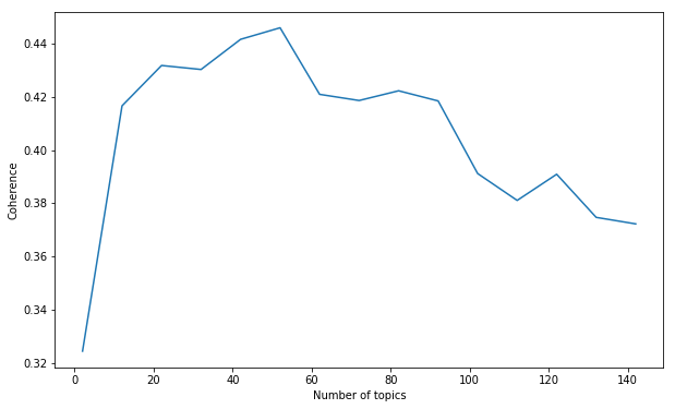
We started by training 15 models at 10-topic intervals: a model with 2 topics, a model with 12 topics, a model with 22 topics, and so on. It looked like the peak coherence was somewhere in the first half of the range:

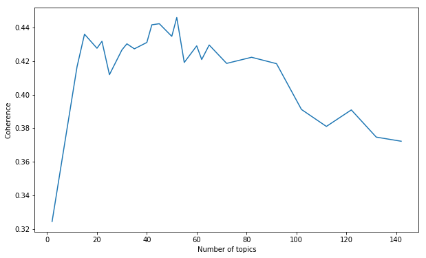
From there, we could refine our search. We trained models at 5-topic intervals from 15 up to 70:

After a few more iterations, we found the coherrence peaked at 52 topics.

The topics

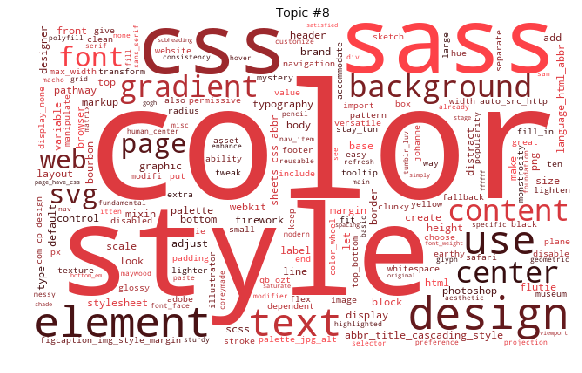
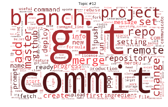
Since a topic consists of a list of words, weighted by the probability they occur in a document that is about the topic, we can use those words and weightings to generate word clouds! The topics aren’t all easy to understand, as is usually the case with a topic model, but there are some which show a very clear theme.

From topics to recommendations

After all this work we had a topic model, but we still didn’t have recommended posts on the blog!

When we run a new post through the topic model, we get a vector of 52 values representing how strongly correlated the post is to each topic. To find similar posts, we need to find posts that have similar topic distributions.

We do this using the Jensen-Shannon distance, which is a popular measure for the similarity of two probability distributions. The recommendations you see at the end of every post are the three posts whose topic distribution has the smallest Jensen-Shannon distance from the topic distribution of the post you just read.

When our blog engine imports new content from GitHub, it now requests new recommended posts from our topic modelling app, which we called Sommelier. It takes a minute or two to build a new model and calculate the J-S distance between each pair of posts, so Sommelier does that work in the background using Celery and posts the results back to the blog engine to be stored in its database.

Acknowledgements

• Rachel Brynsvold’s PyTexas 2017 talk is where I first learnt about topic modelling.
• killerT2333’s Kaggle Notebook is where I learnt about using Jensen-Shannon distance to compare topic vectors.

The moment of truth

Having reached the end of this post, you’re about to see the topic recommendation system in action. Check out the (probably!) related posts below—how do you think the model did?