Neural nets are a common buzzword when it comes to the modern world of programming and machine learning. But what is a neural net? Why is it talked about so much? How does it work? First of all, if you are completely new to machine learning I recommend our introduction to machine learning which offers a great general overview.
A neural net is, at its core, a flexible program that can be adapted to solve many different problems. There are two phases to using a neural net: first it is trained to recognize patterns in data to solve a specific problem, and then it can be given new examples of the problem and come up with the right answers. It is roughly modeled off the way a human brain works. It consists of layers of nodes that have numeric weights and biases associated with them. As we feed data and expected answers into this network, we slowly adjust these weights, giving us better answers over time until the results converge on something good enough to use in production. This can be used for a large variety of problems, anywhere from recognizing dogs in pictures, to training a bot to play a video game, to learning to translate text. The neural net is behind all of these technologies.
A simple neural net might look something like this:

At a high level we will feed in inputs as i1, i2, i3 and it will output an answer in the form of o1 and o2. We call i1, i2, and i3 the input layer and call o1, and o2 the output layer. Any layer in between (in this case layer 2) is called a hidden layer. Each arrow will have a value associated with it called the weight. This number will determine the importance of that arrow and will be updated over time. b1 is the bias for the hidden layer. Instead of influencing a single node as a weight does it is applied to everything in the layer. b2 is also a bias and is a value to influence the whole output layer.
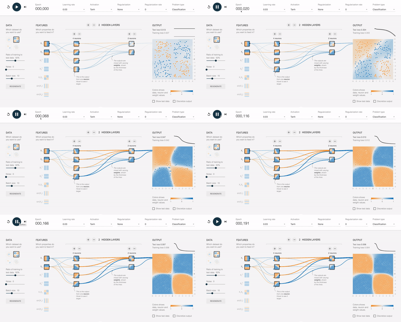
We will initialize each of these arrows with random weights. We then feed in training data multiplying the inputs by the weights to scale them by importance. We then sum these products per the node they came from. We take the result of this and treat is as a probability of being a certain result. So the diagram above could have o1 be probability that a picture contains a dog and o2 could be probability that a picture contains a cat. That way we could see if an image contains either a cat, a dog, or both. We then compare it to the expected answer and calculate the error between the expected and the actual. We can then use this error to determine how weights should be adjusted. This is done through a process called backpropagation. This uses the chain rule and treats every node in the neural net as a mathematical function, taking the partial derivative with respect to the whole and finding how much effect the node has on the whole. Using backpropagation we can see in which direction (up or down in this case) we should move each of the weights and biases. A practical example of this in action might look like this:

Notice that given an input of a horizontal divider and a vertical divider, it is able to fit to the expected shape over time. The background color of the output box represents what the network is predicting and the dots themselves are the data that we are feeding in. Also notice that the size of the connecting lines throughout the net are changing over time. This represents how the weights of the inputs are changing as we feed data in. Blue represent positive weights and orange represents negative. You can see that in the hidden layer there are different shapes that are being looked for with different weights attached to them. Then, by combining those shapes with different weights we can get new shapes. In this example we have several negative and positive lines of pretty equal strength going into the final layer and also have the top output layer with a strong positive and three strong negatives. However we can also have more straightforward example like this:

Here we reach the result much faster and it’s clear that some of the shapes are being relied upon much more than the others. Feel free to play around with this here.
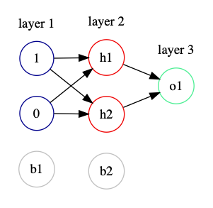
Finally, I want to use the steps described above and walk through a simple and slightly contrived example. Let’s say we want to train a neural net to tell if a number is even. It could look like this

Where the inputs are the binary representation of the number. We will have a 1 represent true (that a number is even) and a zero represent false (that a number is odd). So if the answer is closer to 1 that means it has a higher probability of being even and if it’s closer to 0 it has a higher probability that it’s odd. Let’s examine what a single forward pass of this network looks like. We start by randomly initializing the weights of the neural net as well as biases.

The actual equation for calculating the hidden layer with these weights is:

With the inputs transposed so it’s 1 x 2 matrix instead of a 2 x 1 vector, which when worked out would also look like this:


Once we have calculated these values, we want to scale them to ensure that they will be between zero and one. This is not technically necessary here because our inputs will always be either 0 or 1, but for teaching purposes I will walk through it. In this case we will be using the logistic function, which looks like this:

We use this function to scale h1 and h2:


We then use these with the values of h1 and h2 to provide us the correct answer. We do the same process to find o1.

Once again we transpose the result from last time and end up getting our result. After applying the logistic function to that 0.73681285 we get 0.676298522. This is our prediction. 0.676298522 is closer to 1 than zero. So we are predicting based on our randomized weights that the number one is even. Note the closer we are to 1 or 0 the stronger we are claiming the probability of being that respective answer is. So this is not a strong prediction. Obviously this is not correct. However, we have made a prediction. This concludes the forward pass of our neural net. From here we calculate the error given the expected answer and the prediction and adjust weights based on this answer. I will not delve into the backward pass in this article, but if you are interested this is a great place to get started.
Included are some links that are great resources for learning more about machine learning:
A Step By Step Backpropagation Example
Under The Hood Of Neural Network Forward Propagation - The Dreaded Matrix Multiplication

